| New Products & Service | FEM Analysis | ||||||||
●Price Ultimate: USD21,000 ●ReleaseApril 2021 |
|||||||||
|
Overview The following functions have been added to Engineer's Studio® Ver.10.
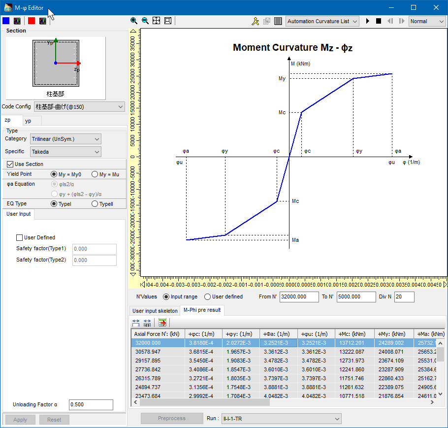
Both functions can be applied to uniaxial bending but not to biaxial bending. Use the fiber element for the biaxial bending M-φ element that takes into account the influence of change in axial force As for M-φ characteristics automatically created from sections, input the maximum and minimum value and the number of changing axial force in the M-φ Tables or M-φ Thumbnails in "Model Properties | M-φ Element Properties". Then press "Preprocess" button to calculate the same number of M-φ characteristics as the input number of axial force (Fig.1). To calculate arbitrary M-φ feature that is not calculated from section automatically, input M and φ the same number as axial force directly.
When the FEM analysis is performed, M-φ features of each axial force are taken into account at the same time. The figure 2 is an example of an analysis of the case of 3 axial forces. M-φ characteristics when the axial force is N1, N2, and N3 are available.
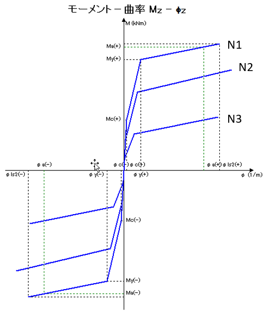
When a load is applied, in a step, all the three M-φ characteristics are updated at the same time as shown in Fig. 3 and reach the point A, B, and C. For example, when a new axial force acquired at that step is between N1 and N2, the linear interpolation is applied between A and B and creates a new bending moment and rigidity.
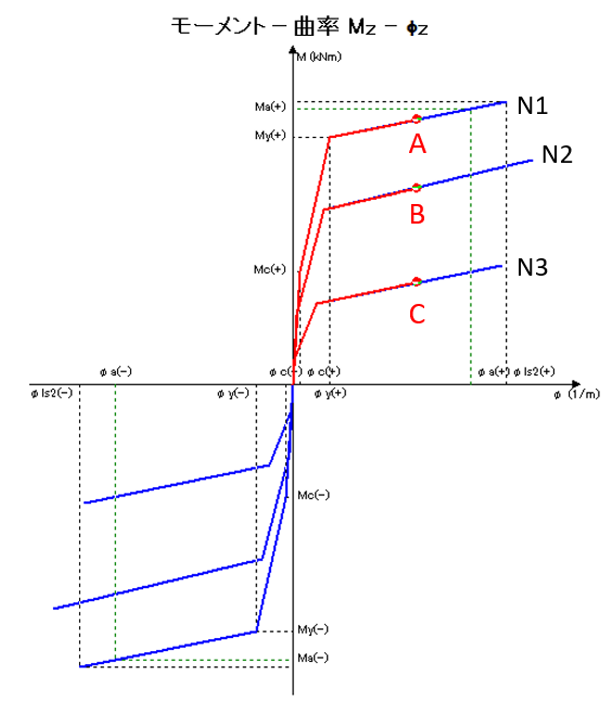
The unloading is handled in the same way. In a step, all the three M-φ characteristics are updated coinsidently as shown in Fig. 4 and reach the point D, E, and F. For instance, when a new axial force acquired at that step is between N1 and N2, the linear interpolation is applied between D and E and creates a new bending moment and rigidity.
M-θ Model (Spring Element) That Takes Into Account the Influence of Change in Axial Force Handled in the same way as M-φ element above that is taking into account changes in the axial force. Others Response value and verification value that take into account changes in the axial force is also calculated for the curvature verification, plasticity rate verification (2012 specifications), residual displacement verification, and displacement verification (2017 specifications). |
|||||||||
| (Up&Coming '21 Spring issue) |
|
|

